What is OpenCV ?
OpenCV is a C library designed to help with computer vision programs. It provides many inbuilt functions that are mainly aimed at real time image processing. It has several hundreds of image processing and computer vision algorithms, which make developing advanced computer vision applications easy and efficient. It includes image filtering, image transformations, color space conversions, contour detection, object tracking algorithms etc. What are contours ? Contours can be explained simply as a curve joining all the continuous points (along the boundary), having same color or intensity. So if we find a contour in a binary image, we are finding the boundaries of objects in an image. That is why, OpenCV doc says, “The contours are a useful tool for shape analysis and object detection and recognition“.
Contour detection :
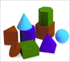
Lets see how to detect contours of particular color. Here I have done for blue color.
Input image :-

Following steps are needed :
1. Color space conversion :
A good first step in many CV algorithms is to convert the image to HSV. HSV stands for Hue, Saturation and Value/Brightness. This makes picking out objects based on color’s a bit simpler. OpenCV has cvtColor function for conversion. Imgproc.cvtColor( mRgbMat, mHsvMat, Imgproc.COLOR_RGB2HSV, channelCount );
Parameters :
a. mRgbMat – Input RGB image.
b. mHsvMat – Output HSV image.
c. Imgproc.COLOR_RGB2HSV – Color space conversion code.
d. channelCount – Number of channels in destination image.
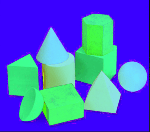
After HSV conversion,

2. Image Processing :
Preprocess the image to select all pixels within specified range of color. We’ll do this based purely on their HSV values. OpenCV provides InRange function that can be used to pick out pixels based on their values. We provide upper and lower threshold values to this function, it then generates a mask; a binary image where foreground pixels (white) are within the specified range. We can specify range manually(like I have used constant values) or you might also use one of the OpenCV machine learning algorithms to pick the ranges automatically. Scalar lowerThreshold = new Scalar ( 120, 100, 100 ); // Blue color – lower hsv values Scalar upperThreshold = new Scalar ( 179, 255, 255 ); // Blue color – higher hsv values Core.inRange ( mHsvMat, lowerThreshold , upperThreshold, mMaskMat );
Parameters :
a. mHsvMat – Input HSV image.
b. lowerThreshold – Lower threshold values.
c. upperThreshold – Upper threshold values.
d. mMaskMat – Output masked image which contains pixels in specified range.
3. Performing morphological operations :
We then perform morphological operations like dilation or erosion which helps in removing noise in the mask. Dilation and erosion are two fundamental morphological operations. Dilation adds pixels to the boundaries of objects in an image, while erosion removes pixels on object boundaries.(ref.Morphological operation) . Imgproc.dilate ( mMaskMat, mDilatedMat, new Mat() );
Parameters :
a. mMaskMat – Input image.
b. mDilatedMat – Output dilated image.
c. new Mat() – Kernel mat.
4. Finding contours :
The function FindContours() computes contours from binary images. Imgproc.findContours ( mDilatedMat, contours, hierarchy, Imgproc.RETR_LIST, Imgproc.CHAIN_APPROX_SIMPLE );
Parameters :
a. mDilatedMat – Source, an 8-bit single-channel image. Non-zero pixels are treated as 1’s. Zero pixels remain 0’s, so the image is treated as binary,
b. contours – Detected contours. Each contour is stored as a vector of points.
c. hierarchy – Optional output vector, containing information about the image topology. It has as many elements as the number of contours.
d. mode – Contour retrieval mode .
i) CV_RETR_EXTERNAL retrieves only the extreme outer contours. It sets hierarchy[i][2]=hierarchy[i][3]=-1 for all the contours.
ii) CV_RETR_LIST retrieves all of the contours without establishing any hierarchical relationships.
iii) CV_RETR_CCOMP retrieves all of the contours and organizes them into a two-level hierarchy. At the top level, there are external boundaries of the components. At the second level, there are boundaries of the holes. If there is another contour inside a hole of a connected component, it is still put at the top level.
iv) CV_RETR_TREE retrieves all of the contours and reconstructs a full hierarchy of nested contours. This full hierarchy is built and shown in the OpenCV contours.c demo.
e. Method – Contour approximation method .
i) CV_CHAIN_APPROX_NONE stores absolutely all the contour points. That is, any 2 subsequent points (x1,y1) and (x2,y2) of the contour will be either horizontal, vertical or diagonal neighbors, that is, max(abs(x1-x2),abs(y2-y1))==1.
ii) CV_CHAIN_APPROX_SIMPLE compresses horizontal, vertical, and diagonal segments and leaves only their end points. For example, an up-right rectangular contour is encoded with 4 points.
iii) CV_CHAIN_APPROX_TC89_L1,CV_CHAIN_APPROX_TC89_KCOS applies one of the flavors of the Teh-Chin chain approximation algorithm. 5. Drawing the contours : With the set of contours detected, we can classify these contours and eliminate those that do not meet certain characteristics such as size or morphology. As a result, contours which meet these conditions are drawn in a new image. In this new image only the regions (or contours) interesting or useful for our case will appear, so our analysis will be easier after this classification.
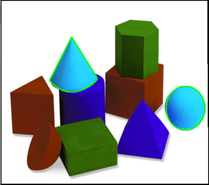
Let’s take a look at following example : for ( int contourIdx=0; contourIdx < contours.size(); contourIdx++ ) { if(contours[contourIdx].size()>100) // Minimum size allowed for consideration { Imgproc.drawContours ( mRgbMat, contours, contourIdx, colorGreen, iLineThickness); } }
An image containing the interesting contours will be generated.
Parameters :
a. mRgbMat – Destination image.
b. contours – Input contours. Each contour is stored as a point vector.
c. contourIdx – Parameter indicating a contour to draw. If it is negative, all the contours are drawn.
d. color – Color of the contours.
e. thickness – Thickness of lines the contours are drawn with. If it is negative (for example, thickness=CV_FILLED), the contour interiors are drawn.
Output image :

